by Hongyu Xiao

Introduction to SeisBench

Welcome to this introductory tutorial on SeisBench! SeisBench is a powerful open-source framework for machine learning in seismology. It provides tools for data loading, processing, model training, and evaluation.

In this notebook, we will cover the basics of loading and inspecting seismological data using SeisBench.

Importing SeisBench

The first step is to import the necessary modules from SeisBench. The `seisbench.data` module contains functionalities for accessing and managing seismological datasets.

# Install SeisBench using pip. 
!pip install seisbench

Loading a Dataset

SeisBench provides access to several pre-compiled datasets. These are curated collections of seismic waveforms and associated metadata, ready for use in machine learning applications. You can find a list of available datasets in the [SeisBench documentation](https://seisbench.readthedocs.io/en/stable/pages/benchmark_datasets.html).

Here, we will load the "ethz" dataset, which is a popular benchmark dataset in seismology. We specify a `sampling_rate` of 100 Hz, which means the waveforms will be resampled to this frequency if they are not already.

import seisbench
import seisbench.data as sbd

data = sbd.ETHZ(sampling_rate=100)
train, dev, test = data.train_dev_test()

2025-09-29 10:40:08,238 | seisbench | WARNING | Check available storage and memory before downloading and general use of ETHZ dataset. Dataset size: waveforms.hdf5 ~22Gb, metadata.csv ~13Mb
2025-09-29 10:40:08,480 | seisbench | WARNING | Component order not specified, defaulting to 'ZNE'.
2025-09-29 10:40:08,480 | seisbench | WARNING | Component order not specified, defaulting to 'ZNE'.

Inspecting the Data

The data object we created is a WaveformDataset. It contains metadata about the entire dataset, such as the number of waveforms and the available data splits (e.g., training, testing, validation). The metadata attribute is a pandas DataFrame that provides a detailed overview of the dataset content.

# Configure pandas to display all columns of a DataFrame
pd.set_option('display.max_columns', None)

# Convert the metadata to a pandas DataFrame for easier inspection
df = data.metadata
# Display the first few rows of the DataFrame
df.head()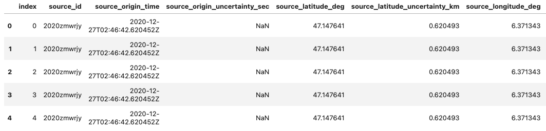

The .streams attribute of the dataset gives you access to the raw waveform data, organized into "streams". In seismology, a stream is a collection of traces. A trace is a single time series of seismic data from one sensor component (e.g., vertical, north-south, east-west).

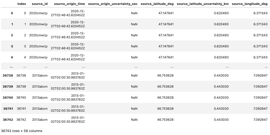
# Display the entire metadata DataFrame
df

# Print the column names to identify the 'station_network_code' field
print(df.columns)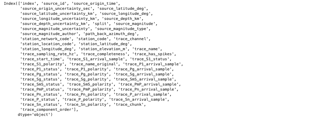

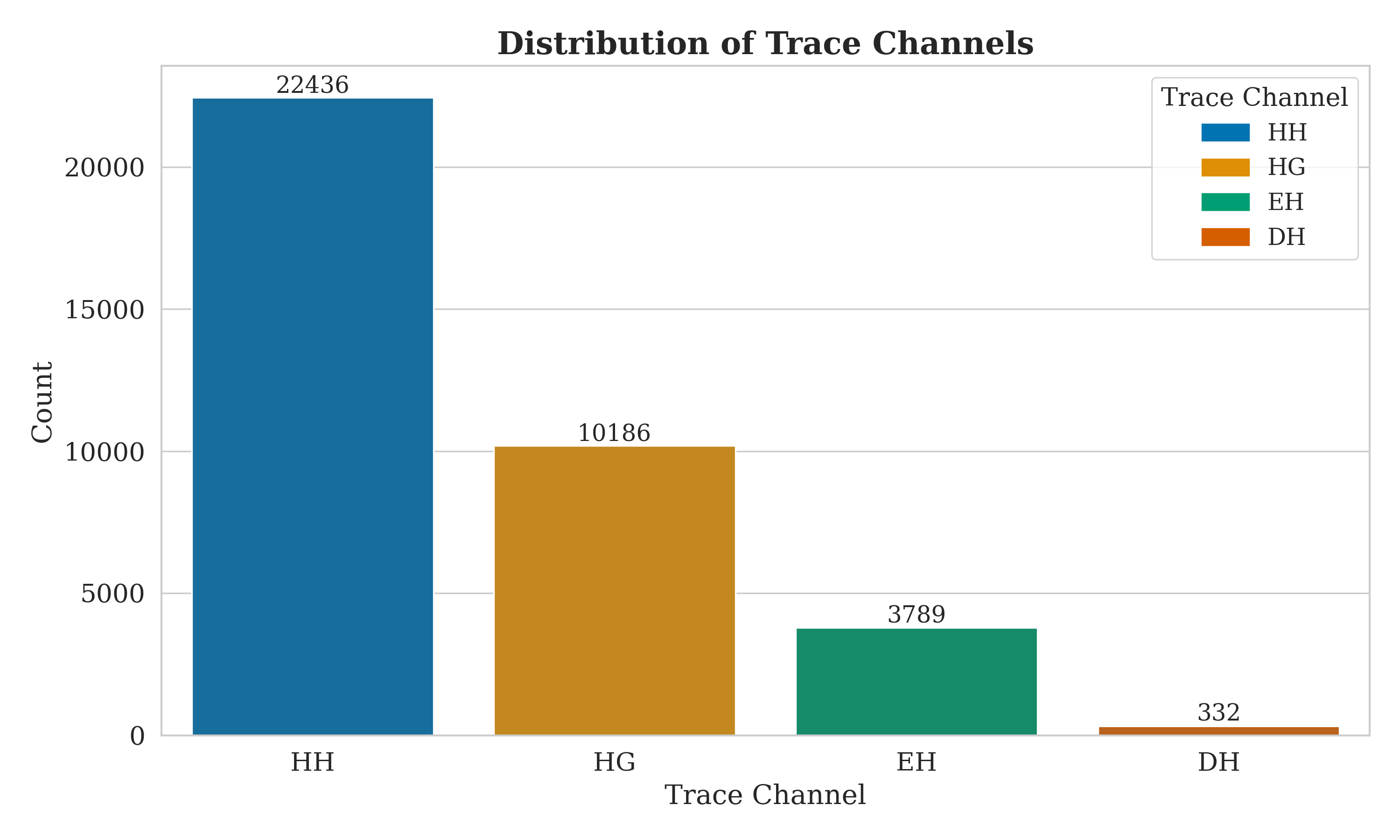
Visualizing the Dataset

Lets start by visualizing the properties of the dataset.

import matplotlib.pyplot as plt
import seaborn as sns
import matplotlib.patches as mpatches

# Set the style 
sns.set_style("whitegrid")
sns.set_context("paper", font_scale=1.5)
plt.rcParams['font.family'] = 'serif'

# Extract the 'trace_channel' column
column_data = df['trace_channel']

# Count the occurrences of each unique value in the column
counts = column_data.value_counts()

# Create a figure and axes
plt.figure(figsize=(10, 6))

# Create the bar plot using a color-blind friendly palette
palette = "colorblind"
ax = sns.barplot(x=counts.index, y=counts.values, palette=palette)

# Add labels and title with increased font size for clarity
ax.set_xlabel('Trace Channel', fontsize=14, fontfamily='serif')
ax.set_ylabel('Count', fontsize=14, fontfamily='serif')
ax.set_title('Distribution of Trace Channels', fontsize=16, fontweight='bold', fontfamily='serif')

# Adjust tick label font
for label in ax.get_xticklabels():
    label.set_fontfamily('serif')
for label in ax.get_yticklabels():
    label.set_fontfamily('serif')

# Add the count values on top of the bars for precise data representation
for i, v in enumerate(counts.values):
    ax.text(i, v + 0.1, str(v), ha='center', va='bottom', fontsize=12, fontfamily='serif')

# Create legend
legend_patches = [mpatches.Patch(color=sns.color_palette(palette)[i], label=l) for i, l in enumerate(counts.index)]
plt.legend(handles=legend_patches, title='Trace Channel', fontsize=12, title_fontsize=13)

# Ensure tight layout and save the figure in high resolution
plt.tight_layout()
plt.savefig("trace_channel_distribution.png", dpi=300)
plt.show()